TD4 - Spectral Analysis and Filtering
from __future__ import division
import numpy as np
import scipy.fftpack as sf
import matplotlib.pyplot as plt
import math
import pylab as pl
import scipy.signal as sig
from scipy import misc
1. STFT (Short Time Fourier Transform) and source separation.
In this part, we use STFT which is a collection of Fourier transform of a 1D signal on time subintervals. Why using STFT ?
The length of a music signal for 4 minutes sampled at a rate of 44kHz is roughly \(2500*44000 \simeq 1.1 \times 10^7\).
The length of a music note is of the order of a tenth of a second.
Conclusion: do not use FFT on the whole signal but on short segments of it.
We use it in order to experiment source separation which comes from the idea that the different signals may present very different behaviour in the frequency domain.
# utils to load the sounds.
import numpy as np
import wave as wv

def load_sound(file, n0):

    x_raw = wv.open(file)
    n = x_raw.getnframes()
    x = np.frombuffer(x_raw.readframes(-1), 'Int16')
    x_raw.close()

    if file[::-1][:8][::-1] == "bird.wav":
        x = np.delete(x,list(range(6001)) + list(range(12500, 15001)) + list(range(22500, 24001)) + list(range(32500,34001)))

    if n0 !=0 and n0 < n:
        x = x[:n0]

    return x/np.max(x)
Hereafter, we load the \(3\) sounds and plot the second one.
n = 1024*16
s = 3 #number of signals.
x = np.zeros([n,3])
x[:,0] = load_sound("bird.wav",n)
x[:,1] = load_sound("female.wav",n)
x[:,2] = load_sound("male.wav",n)

## listen to a sound.
from IPython.display import Audio
Audio(x[:,1], rate = 15000)
/opt/hostedtoolcache/Python/3.7.9/x64/lib/python3.7/site-packages/ipykernel_launcher.py:9: DeprecationWarning: Numeric-style type codes are deprecated and will result in an error in the future.
  if __name__ == '__main__':
# Show the numerical signal.
x = x/np.tile(np.std(x,0),(n,1))
p = 2 #number of micros
import matplotlib.pyplot as plt
plt.figure(figsize = (10,10))
plt.xlim(0,n)
plt.plot(x[:,2])
plt.show()
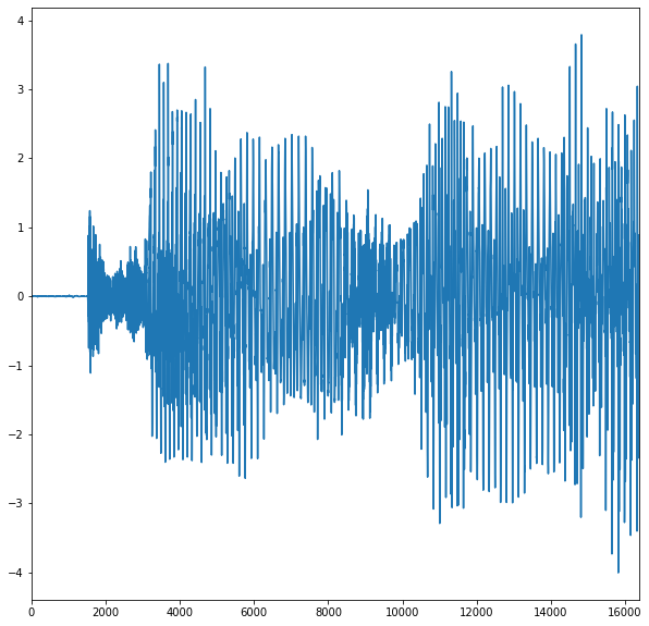
We simulate two micros which are implemented by linear combinations of the signals.
theta = np.linspace(0, np.pi, s + 1)[:-1]
theta[0] = .2
print("theta:", theta)
M = np.vstack((np.cos(theta), np.sin(theta)))
## recorded signals
mixedSignals = np.dot(x, M.T)
print("length of the signals", np.shape(mixedSignals))
# Listen to the two recorded signals.
from IPython.display import Audio
Audio(mixedSignals[:,1], rate = 15000)
theta: [0.2        1.04719755 2.0943951 ]
length of the signals (16384, 2)
### We use the STFT function from the python package signal and plot it.
import scipy.signal as sig
plt.figure(figsize = (15,15))
for i in range(x.shape[-1]):
    f,t,w = sig.stft(x[:,i])
    plt.subplot(1,x.shape[-1],i+1)
    plt.title(f"stft of signal {i}")
    plt.imshow(np.log(np.abs(w)))
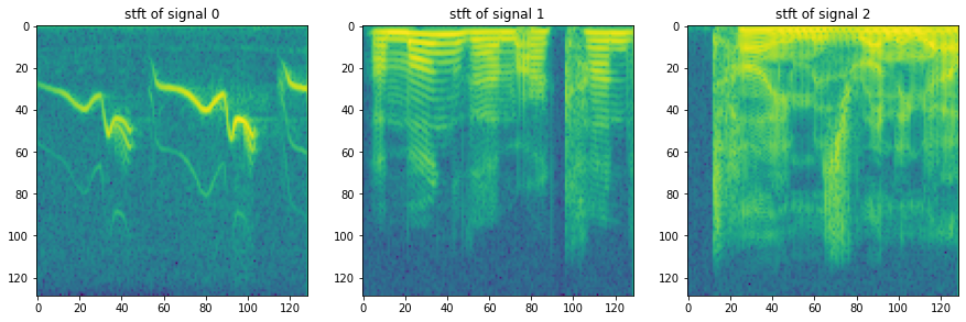
We numerically check that the STFT and ISTFT are indeed inverse from each others.
[micro1, micro2] = mixedSignals.T # destructuring

stft = lambda im : sig.stft(im,noverlap = 64,nperseg = 128)
istft = lambda im : sig.istft(im,noverlap = 64,nperseg = 128)

f,t,w1 = stft(micro1)
f,t,w2 = stft(micro2)
print('w1:', w1.shape, ' w2:', w2.shape)
W = np.asarray([w1.flatten(),w2.flatten()])
print('W(',W.shape,'):', W)
t,recov = istft(w1)
print(np.sum((micro1 - recov)**2))
w1: (65, 257)  w2: (65, 257)
W( (2, 16705) ): [[ 1.16144549e-02+0.j  1.61385888e-02+0.j  1.85006418e-02+0.j ...
   1.18385135e-04+0.j  7.66135211e-04+0.j  4.97046266e-03+0.j]
 [ 2.27491165e-03+0.j  6.23925565e-03+0.j  4.34767210e-03+0.j ...
  -3.85635906e-05+0.j  2.08275687e-04+0.j  2.12086109e-03+0.j]]
1.1214543788890096e-27
By selecting randomly a group of points in time, we plot in the plane the coordinates of the points, being the measured signals by the micros.
from random import shuffle
nbre_selec = 3000

def extractSomeValues(x, nb = 600): # along first axis
    randomId = np.arange(x.shape[0])
    shuffle(randomId)
    return x[randomId[:nb]]

print(mixedSignals.shape[0])

ySamples = extractSomeValues(mixedSignals, nbre_selec)
plt.plot(ySamples[:,0],ySamples[:,1],"o",markersize=1)
plt.show()
16384
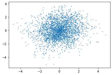
Q1: Do the same with the STFT signals, what do you observe ?
# W represent STFT signals

signal = W
#to have it in the good axis
signal = signal.T
#use on real part
signal = signal.real


stftSamples = extractSomeValues(signal, nbre_selec)
plt.plot(stftSamples[:,0],stftSamples[:,1],"o",markersize=1)
plt.show()
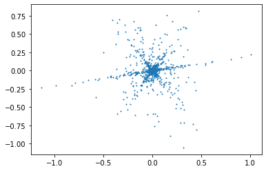
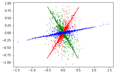
We observe that points congregates to 3 distincts lines that cross at a central point (the origin).
Q2: For each point in the plot above, compute its angle (angle between 2 points) and plot the distribution of the angles (use the function np.histogram) and plot it.
 #math.atan2() : Returns the tangent(y,x) in radius

pts = np.dstack((stftSamples[:,0],stftSamples[:,1]))[0]

angles = np.array([np.arctan2(p[1],p[0]) for p in pts])
angles = angles % np.pi #take angle between 0 and pi

resolution = 200
plt.figure(figsize=(20,10))
plt.title("Angles distribution")
histogram = plt.hist(angles, bins=resolution)
plt.show()
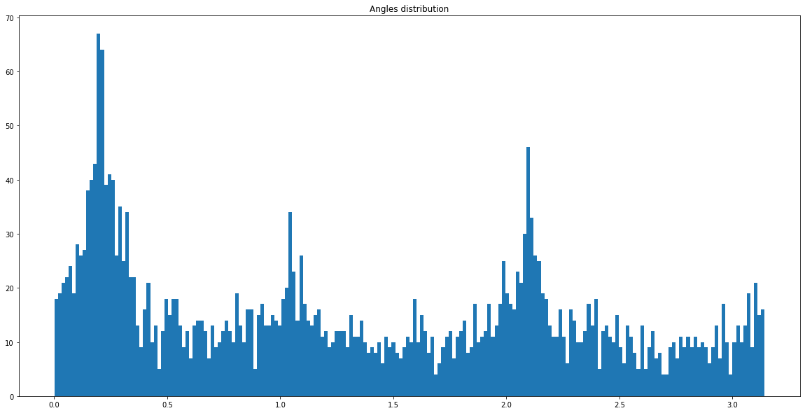
Q3: By selecting the highest peaks of the distribution, estimate the angles of the mixing.
#A bin is range that represents the width of a single bar of the histogram along the X-axis
peakCounts, peakBins = np.histogram(angles, bins= resolution)
#np.histogram computes the occurrences of input data that fall within each bin
#which in turns determines the area (not necessarily the height if the bins aren't of equal width) of each bar.

peaks, prop = sig.find_peaks(peakCounts, distance=10)
plt.plot(peakBins[peaks], peakCounts[peaks])
plt.show()

# sort by argument in order to find our maximal peaks
# ([-3:]) is used to keep only the first three maximum values
maxPeakIdx = peakCounts[peaks].argsort()[-3:]

peakAngles = peakBins[peaks][maxPeakIdx]
print("Angles : ", peakAngles)
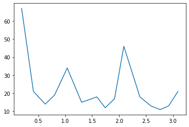
Angles : [1.03679751 2.08905214 0.18871168]
Q4: Using the STFT recorded signals, take each point in the plane and compute its projection on each recovered directions. It gives a vector of 3 estimated projections.
#https://stackoverflow.com/questions/9605556/how-to-project-a-point-onto-a-plane-in-3d
#https://gamedev.stackexchange.com/questions/72528/how-can-i-project-a-3d-point-onto-a-3d-line

print("peakAngles:", peakAngles)
directions = np.array([[math.cos(angle), math.sin(angle)] for angle in peakAngles])
directions = np.array([d / np.linalg.norm(d) for d in directions]) # normalize
print("directions:", directions)

# using the formula : A + dot(AP,AB) / dot(AB,AB) * AB
# where A is the origin (0, 0)
# dir is our B normalized
projections = np.array([[np.dot(pt, d)*d for d in directions] for pt in signal])
print("projections.shape:", projections.shape)

plt.plot(projections[:,:, 0],projections[:,:,1],"o",markersize=1)
plt.show()
peakAngles: [1.03679751 2.08905214 0.18871168]
directions: [[ 0.5089795   0.86077864]
 [-0.49536574  0.86868451]
 [ 0.98224673  0.1875936 ]]
projections.shape: (16705, 3, 2)
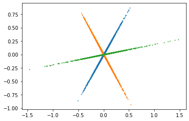
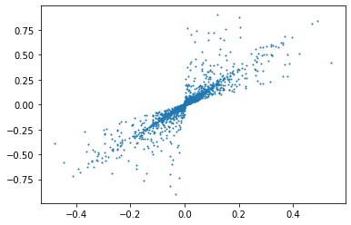
Q5: For each frequency point in the signal STFT, select the direction on which it has the largest projection. And threshold using the code below.
projectionsStrength = np.array([[np.abs(np.dot(pt, d)) for d in directions] for pt in signal])
bestProjection = np.argmax(projectionsStrength, axis=1)

extracted = [[], [], []]
for b, pt in zip(bestProjection, signal):
    extracted[b].append(pt)

extracted = [np.array(a) for a in extracted] # convert to numpy array
# print(extracted[0].shape, extracted[1].shape, extracted[2].shape)

#display helpers
directionLines = np.array([[-d, d] for d in directions]) # for line display
color = ['r', 'g', 'b']

for i in range(len(extracted)):
    plt.plot(extracted[i][:, 0],extracted[i][:, 1],"o",markersize=1, c=color[i])
    plt.plot(directionLines[i][:, 0], directionLines[i][:, 1], c=color[i]) # Red straight line
# set values to zero for non selected values
splitted = np.array([(np.where(bestProjection == i, 1, 0)*signal.T).T for i in range(3)])
print(splitted.shape)
plt.plot(extracted[0][:,0],extracted[0][:,1],"o",markersize=1)
plt.show()
(3, 16705, 2)
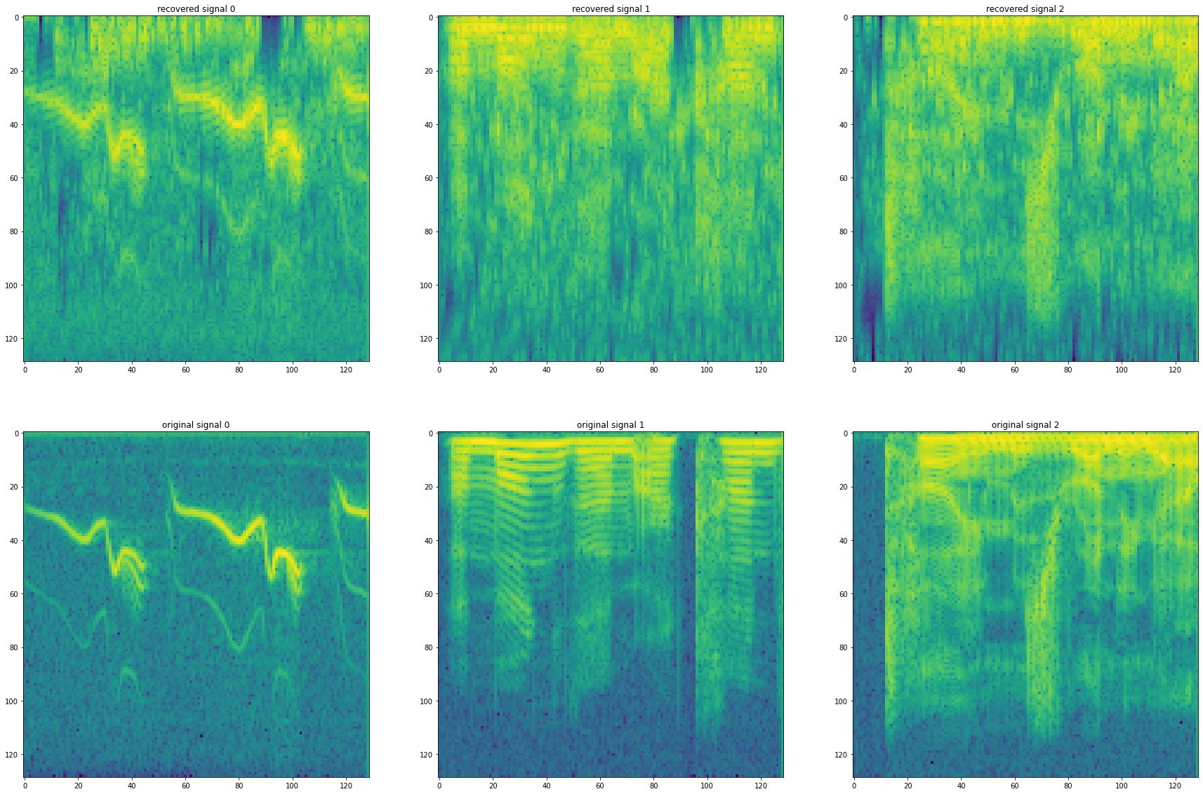
Q6: Plot the STFT and the time domain of the recovered signals and the original signals. Estimate the performance using the SNR implemented below.
def snr(x, y):
    s =  np.linalg.norm(x - y)
    if s == 0:
        return "Equal inputs"
    return 20 * np.log10(np.linalg.norm(x) /s)

t, recov = istft(splitted[2][:, 0].reshape(65, 257))

recoveredSignals = np.array([istft(s[:, 0].reshape(65, 257)) for s in splitted])[:, 1]

# fix order to match original order in variable x
recoveredSignals = recoveredSignals[[2, 0, 1]]

plt.figure(figsize = (30,20))
for i in range(x.shape[-1]):
    f,t,w = sig.stft(recoveredSignals[i])
    plt.subplot(2,x.shape[-1],i+1)
    plt.title(f"recovered signal {i}")
    plt.imshow(np.log(np.abs(w)))

    f,t,w = sig.stft(x[:, i])
    plt.subplot(2,x.shape[-1],x.shape[-1]+i+1)
    plt.title(f"original signal {i}")
    plt.imshow(np.log(np.abs(w)))

for i in range(x.shape[-1]):
    print(f'snr signal {i}: {snr(recoveredSignals[i], x[:, i])}')
snr signal 0: -0.9000975306507928
snr signal 1: -9.422646487613866
snr signal 2: -12.272112093209152
Q7: Listen to the reconstructed signals and the original signals.
i = 0
from IPython.display import Audio
Audio(recoveredSignals[i], rate = 15000)
i = 0
from IPython.display import Audio
Audio(x[:,i], rate = 15000)
2. The goal of this part is to explore implementations of a FIR or an IIR.
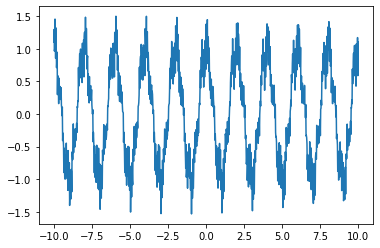
We plot below a signal with a mix of low and high frequencies.
f = lambda t: np.cos(np.pi*t) + 0.2*np.sin(5*np.pi*t+0.1) + 0.2*np.sin(30*np.pi*t)  + 0.1*np.sin(32*np.pi*t+0.1) + 0.1*np.sin(47* np.pi*t+0.8)
t=np.linspace(-10,10,1000)
signal=f(t)
print(np.shape(t),np.shape(signal))
plt.plot(t, signal)
(1000,) (1000,)
[<matplotlib.lines.Line2D at 0x7fc24fe32390>]
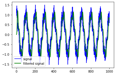
Q1. Implement an ideal low pass filter using Fourier transform in 1D:
Compute the inverse FFT of a low pass filter and cut it with a window that will be passed in argument and apply it to the signal above by convolution or using FFT.
order = 5
sampling_freq = 30
cutoff_freq = 2
sampling_duration = 5
number_of_samples = sampling_freq * sampling_duration
normalized_cutoff_freq = 2 * cutoff_freq / sampling_freq

numerator_coeffs, denominator_coeffs = sig.butter(order, normalized_cutoff_freq)

filtered_signal = sig.lfilter(numerator_coeffs, denominator_coeffs, signal)

plt.plot(signal, 'b-', label='signal')
plt.plot(filtered_signal, 'g-', linewidth=2, label='filtered signal')
plt.legend()
<matplotlib.legend.Legend at 0x7fc24fd90490>
Q2. Using the code below, implement an IIR filter defined by its numerator which will be set to a constant \(b\) and its denominator which will be set to \(1-az^{-1}\).
What can you say about the range of the parameter \(a\) in order to obtain a stable filter. Experimentally, determine the ranges of \(a\) to get respectively a low-pass filter and a high-pass filter. Give a theoretical explanation.
\(z^{-1} = \frac{Z^{-1}}{a − a_Z}\)
def myIIR(x,a,b):
    ### a is the numerator
    ### b is the denominator
    assert(len(a)==len(b)),"a,b must have the same length"
    y = np.zeros_like(x)
    k = len(a)
    for i in range(len(a),len(x)):
        y[i] = np.sum(np.flipud(b)*y[i-k:i]) + np.sum(np.flipud(a) * x[i-k+1:i+1])
    return y
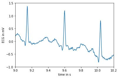
In the following, we are given an electrocardiogram. We plot it as a function of time.
### load the data which is an electrocardiogram which is sampled at 360Hz
ecg = misc.electrocardiogram()
### Different plots.
fs = 360.0
### Since it is sampled at 360Hz, recall that Hz is the number of cycle per second, then the
### time is obtained as follows:
time = np.arange(ecg.size) / fs
### simple plot.
plt.plot(time, ecg)
plt.xlabel("time in s")
plt.ylabel("ECG in mV")
plt.xlim(9, 10.2)
plt.ylim(-1, 1.5)
plt.show()
print("time min", time[0])
print("time max", time[-1])
time min 0.0
time max 299.9972222222222
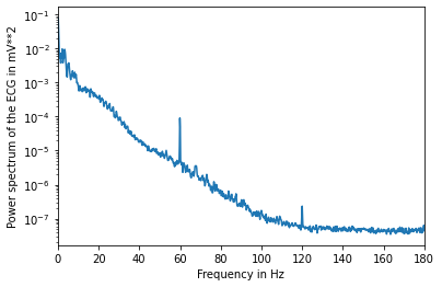
### Use the scipy function to get the power spectrum of the signal.
f, Pxx = sig.welch(ecg, fs=fs, nperseg=2048, scaling="spectrum")
plt.semilogy(f, Pxx)
plt.xlabel("Frequency in Hz")
plt.ylabel("Power spectrum of the ECG in mV**2")
plt.xlim(f[[0, -1]])
plt.show()
Q3. Estimate the number of heartbeats in the following electrocardiogram and estimate the mean value of the interval between two heartbeats. You can use the method of your choice. A possible method consists in using a band pass filter and then extract the maximum values of the filtered signal.
import statistics

fL = 0.1  # Cutoff frequency as a fraction of the sampling rate (in (0, 0.5)).
fH = 0.4  # Cutoff frequency as a fraction of the sampling rate (in (0, 0.5)).
b = 0.08  # Transition band, as a fraction of the sampling rate (in (0, 0.5)).

def band_pass():
    N = int(np.ceil((4 / b)))
    if not N % 2: N += 1  # Make sure that N is odd.
    n = np.arange(N)

    # Compute a low-pass filter with cutoff frequency fH.
    hlpf = np.sinc(2 * fH * (n - (N - 1) / 2))
    hlpf *= np.blackman(N)
    hlpf = hlpf / np.sum(hlpf)

    # Compute a high-pass filter with cutoff frequency fL.
    hhpf = np.sinc(2 * fL * (n - (N - 1) / 2))
    hhpf *= np.blackman(N)
    hhpf = hhpf / np.sum(hhpf)
    hhpf = -hhpf
    hhpf[(N - 1) // 2] += 1

    # Convolve both filters.
    return np.convolve(hlpf, hhpf)

h = band_pass()

s = np.convolve(ecg, h)
plt.plot(s)
peaksS, propS = sig.find_peaks(s)

meanVal = statistics.mean(peaksS)
print("Mean value : ", meanVal)
Mean value : 54199
