Inverse Problem¶

In this notebook, I give a simple example of an inverse problem which necessitates regularization.

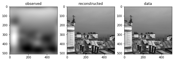
Consider for instance $$I_{observed} = K_\sigma \star I + n$$ where $K_\sigma$ is a gaussian blur and $n$ is a gaussian iid noise. A naive idea consists in inverting $K_\sigma$ in Fourier space. It works when there is no noise, but completely fails in the presence of noise.

from __future__ import division
import numpy as np
import scipy as sp
%matplotlib inline
import scipy.fftpack as ft
%pylab inline

Populating the interactive namespace from numpy and matplotlib

# load an image
import imageio as imio
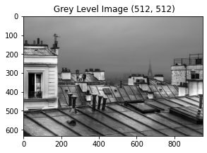
colored_image = imio.imread('toits.jpg')
print(colored_image.shape)
n = colored_image.shape[0]-1
n = 512
image = np.sum(colored_image*[0.21, 0.72 ,0.07],axis=-1)[:n,100:100+n]

plt.figure(figsize = (10,10))
plt.subplot(1,2,1)
plt.gray()
#cropped = image[n:n+64,n:n + 64]
plt.title(" Grey Level Image " + str(np.shape(image)))
cropped = image
plt.imshow(colored_image)
print(np.mean(cropped),np.std(cropped),(np.min(cropped)))
print(image.shape)
image0 = np.copy(image)

(633, 950, 3)
128.55839157104492 50.33679038212257 0.0
(512, 512)

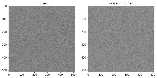
Remark: Noise in Fourier is also a noise. You can guess that the distribution of the energy of the noise in Fourier is similar to its distribution in space.

sigma = 1.0
noise = sigma*np.random.randn(image.shape[0],image.shape[1])
noise_fourier = fft2(noise,norm = "ortho")
plt.figure(figsize = (10,10))
plt.subplot(1,2,1)
plt.gray()
plt.imshow(noise)
plt.title(" noise ")
plt.subplot(1,2,2)
plt.imshow(real(noise_fourier))
plt.title(" noise in fourier ")
print("noise pixels",np.sum(noise**2))
print("noise fourier",np.sum(np.abs(noise_fourier)**2))

noise pixels 262319.45579165744
noise fourier 262319.45579165744

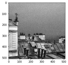
## Add some noise to the image
def clamp(x):
    temp =  255*(x>255) + x * (x<255) 
    return temp * (x>0)

sigma = 20.0
def GaussianNoise(image,sigma):
    return image + sigma*np.random.randn(image.shape[0],image.shape[1])

def SaltNoise(image,sigma):
    return clamp(image + sigma*(np.random.randn(image.shape[0],image.shape[1])>0))

noisy_image  = clamp(image + sigma*np.random.randn(image.shape[0],image.shape[1]))
print(np.min(noisy_image))
plt.imshow(noisy_image)

-0.0

<matplotlib.image.AxesImage at 0x7fe148b13ed0>

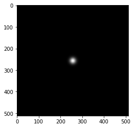
### Construct a gaussian filter.
def construct_gaussian_filter(n,sigma_filter):
    t = np.concatenate((np.arange(0,n/2+1), np.arange(-n/2,-1)))
    [Y,X] = np.meshgrid(t,t)
    h = np.exp(-(X**2+Y**2)/(2.0*sigma_filter**2) )
    h = h/np.sum(h)
    return h
sigma = 10
n = 512
h = construct_gaussian_filter(n,sigma)
imshow(ft.fftshift(h))

<matplotlib.image.AxesImage at 0x7fe148af2b50>

## In Fourier space, convolution is product so 
def myConvPlusNoise(image,sigma_filtre = 0.0,sigma_noise = 0.0):
    w = construct_gaussian_filter(image.shape[0],sigma_filtre)
    temp = real(ifft2(fft2(w)*fft2(image)))
    result= GaussianNoise(temp,sigma_noise) 
    return result

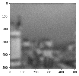
observed_image = myConvPlusNoise(image,sigma_filtre = 10, sigma_noise = 20)
imshow(observed_image)

<matplotlib.image.AxesImage at 0x7fe148a67f90>

### simple inversion using fft
### assume that sigma_filter is known
def naive_deconvolution(image_observed,sigma_filter):
    w = construct_gaussian_filter(image_observed.shape[0],sigma_filter)
    deconv = real(ifft2(fft2(image_observed)/fft2(w))) 
    return deconv

### First test: without noise.

sigma_filtre = 30.0
observed_image = myConvPlusNoise(image,sigma_filtre = sigma_filtre, sigma_noise = 0.0)
reconstructed = naive_deconvolution(observed_image,sigma_filtre)
plt.figure(figsize = (10,10))
plt.subplot(1,3,1)
plt.gray()
plt.imshow(observed_image)
plt.title(" observed ")
plt.subplot(1,3,2)
plt.imshow(reconstructed)
plt.title(" reconstructed ")
plt.subplot(1,3,3)
plt.imshow(image)
plt.title(" data ")

Text(0.5, 1.0, ' data ')

### Second test: with noise.

sigma_filtre = 5.0
observed_image = myConvPlusNoise(image,sigma_filtre = sigma_filtre, sigma_noise = 1)
reconstructed = naive_deconvolution(observed_image,sigma_filtre)
plt.figure(figsize = (10,10))
plt.subplot(1,3,1)
plt.gray()
plt.imshow(observed_image)
plt.title(" observed ")
plt.subplot(1,3,2)
plt.imshow(reconstructed)
plt.title(" reconstructed ")
plt.subplot(1,3,3)
plt.imshow(image)
plt.title(" data ")

Text(0.5, 1.0, ' data ')

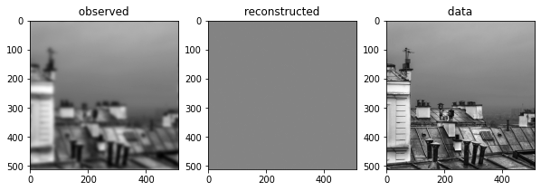
You can observe that, even with a small value of noise, the reconstruction seems to be just noise. Note that the bigger the gaussian width of the gaussian filter, the more sensitive to noise is this reconstruction scheme. The lecture explains why it is the case.

M2 Signal classes

Inverse Problem¶